머신러닝 프로그래밍 12주차 - Binary classification with data Logistic regrsssion

import pandas as pd
import numpy as np
import matplotlib.pyplot as plt

df1 = pd.read_csv("cat1.csv")
df0 = pd.read_csv("cat0.csv")
df1

	entry	event	En1	En2	dt	dr	x1	y1	z1	x2	y2	z2
0	0	1	1.315638	1.804403	151.967212	42.143105	-1304.894054	478.462799	1544.333537	-1157.361908	606.067041	1766.707850
1	1	13	4.827913	2.283814	161.020364	1309.103187	-117.835790	-1464.457077	69.425318	-70.148754	-383.723470	-475.833903
2	2	16	3.011821	2.606455	72.997202	903.456139	1593.153637	-1100.580348	805.977081	1092.321506	-1257.393260	215.991954
3	3	22	3.109662	1.619302	95.681674	246.310774	1414.147550	300.466078	2036.144245	1510.664013	317.401116	2038.324112
4	4	37	2.795250	1.665277	85.430204	452.633419	-1185.771203	-1586.241286	-921.906685	-1048.390809	-1585.937883	-1129.581104
...	...	...	...	...	...	...	...	...	...	...	...	...
9949	9949	99956	1.499017	2.253849	174.517405	938.596974	-1091.980671	1203.741862	-840.761911	-1055.791096	574.858610	-1024.616952
9950	9950	99957	2.705410	2.874333	715.772076	175.621626	950.171373	898.111879	-1897.760471	962.544864	677.295582	-1880.154811
9951	9951	99983	2.943438	2.512821	1179.579896	60.482252	-1437.391692	807.265834	1213.002043	-1571.892213	721.972273	1238.615481
9952	9952	99987	3.082408	2.868833	145.649583	494.576245	-1658.602340	-479.454709	-1472.514450	-1619.486255	-669.457050	-931.362227
9953	9953	99993	3.196240	1.490613	43.678549	213.871359	1165.018820	1386.749830	-722.045299	1158.905657	1062.491877	-889.901928

9954 rows × 12 columns

plt.hist(df0["dt"], bins=100, density=True, histtype="step");
plt.hist(df1["dt"], bins=100, density=True, histtype="step");

output_2_0

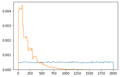
#density - 확률 밀도를 설정하기 위해 가중치 데이터를 정규화한다

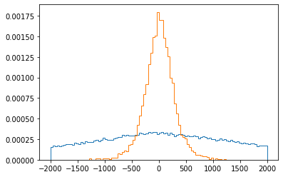
plt.hist(df0["y1"]-df0["y2"], bins=100, range=(-2000,2000), density=True, histtype="step");
plt.hist(df1["y1"]-df1["y2"], bins=100, range=(-2000,2000), density=True, histtype="step");

output_3_0

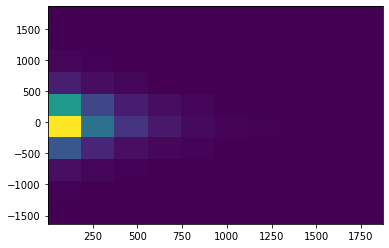
plt.hist2d(df0["dt"], df0["y1"]-df0["y2"]);

output_4_0

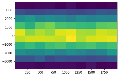
plt.hist2d(df1["dt"], df1["y1"]-df1["y2"]);

output_5_0

df0 = df0[:9000]
df1 = df1[:9000]

# plt.plot 옵션 - https://namyoungkim.github.io/matplotlib/visualization/2017/10/06/visualization/

#markersize	(ms)->마커 크기

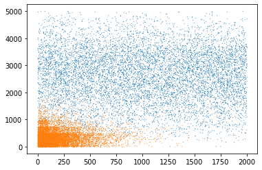
plt.plot(df0["dt"], df0["dr"], '.', ms=0.5)
plt.plot(df1["dt"], df1["dr"], '.', ms=0.5)

[<matplotlib.lines.Line2D at 0x7f4cafacce10>]

output_7_1

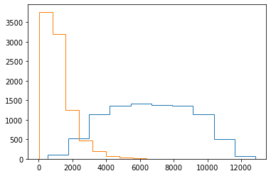
plt.hist(4*df0["dt"]+df0["dr"], histtype="step")
plt.hist(4*df1["dt"]+df1["dr"], histtype="step")

(array([3.766e+03, 3.191e+03, 1.252e+03, 4.780e+02, 1.930e+02, 7.500e+01,
        3.300e+01, 6.000e+00, 4.000e+00, 2.000e+00]),
 array([  15.20712953,  810.57056653, 1605.93400353, 2401.29744052,
        3196.66087752, 3992.02431452, 4787.38775152, 5582.75118852,
        6378.11462551, 7173.47806251, 7968.84149951]),
 <a list of 1 Patch objects>)

output_8_1

#시그 모이 드 함수는 수학적 로지스틱 함수입니다. 통계, 오디오 신호 처리, 생화학 및 인공 뉴런의 활성화 기능에 일반적으로 사용됩니다. 시그 모이 드 함수의 공식은F(x) = 1/(1 + e^(-x))입니다.
def sigmoid(z):
  return 1/(1+np.exp(-z))

def f(x, y, a, b, c):
  return a*x + b*y + c

dts1 = np.array(df1['dt'])/1000
dts0 = np.array(df0['dt'])/1000
drs1 = np.array(df1['dr'])/1000
drs0 = np.array(df0['dr'])/1000
label1 = np.ones(dts1.shape)
label0 = np.zeros(dts0.shape)

dts = np.concatenate([dts1, dts0])
drs = np.concatenate([drs1, dts0])
label = np.concatenate([label1, label0])
data = np.stack([dts, drs, label], axis=1) #가로축으로 합쳐진다
np.random.shuffle(data)

data

array([[0.38524939, 0.06985145, 1.        ],
       [0.03403795, 0.31482386, 1.        ],
       [0.01535261, 0.25602788, 1.        ],
       ...,
       [0.56028966, 0.56028966, 0.        ],
       [0.3714466 , 0.3714466 , 0.        ],
       [0.28964576, 0.28964576, 0.        ]])

def gradF(x, y, a, b, c):
  # 1/(1+np.exp(-z))
  z = f(x, y, a, b, c)
  yy = sigmoid(z)*(1-sigmoid(z))
  # a*x + b*y + c
  da = yy*x
  db = yy*y
  dc = yy*1

  return da, db, dc

losses = []
fitA, fitB, fitC = 1, 1, 1
batchSize = 16
eta = 1e-3
for epoch in range(10000):
  sumLoss = 0.
  nBatch = 0
  for batch in range(0, len(data), batchSize):
    ### Compute loss
    x = data[batch:batch+batchSize+1].T  #DataFrame.transform()는DataFrame에 함수를 적용하고 DataFrame을 변환합니다.
    dt, dr, label = x[0], x[1], x[2]
    z = f(dt, dr, fitA, fitB, fitC)
    z = sigmoid(z)

    df = label - z
    loss = (df**2).mean()

    ### Gradient
    #grad = -2*df*gradF(dt, dr, fitA, fitB, fitC)
    gradA, gradB, gradC = gradF(dt, dr, fitA, fitB, fitC)
    gradA = (df*gradA).mean()
    gradB = (df*gradB).mean()
    gradC = (df*gradC).mean()

    ### parameter update
    fitA = fitA + gradA*eta
    fitB = fitB + gradB*eta
    fitC = fitC + gradC*eta

    ### loss monitor
    #losses.append(loss)
    sumLoss += loss
    nBatch += 1
  losses.append(sumLoss/nBatch)  

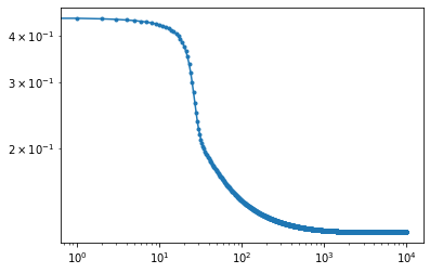
plt.plot(losses, '.-');
plt.yscale('log')
plt.xscale('log')

output_16_0

data0 = data[data[:,2]==0]
data1 = data[data[:,2]==1]

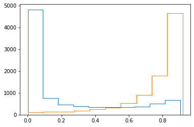
plt.hist(sigmoid(f(data0.T[0], data0.T[1], fitA, fitB, fitC)), histtype='step')
plt.hist(sigmoid(f(data1.T[0], data1.T[1], fitA, fitB, fitC)), histtype='step')

(array([ 101.,  133.,  146.,  177.,  260.,  320.,  527.,  900., 1776.,
        4660.]),
 array([8.41085958e-04, 9.27254960e-02, 1.84609906e-01, 2.76494316e-01,
        3.68378726e-01, 4.60263136e-01, 5.52147546e-01, 6.44031956e-01,
        7.35916366e-01, 8.27800777e-01, 9.19685187e-01]),
 <a list of 1 Patch objects>)

output_18_1

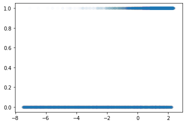
plt.plot(f(data.T[0], data.T[1], fitA, fitB, fitC), data.T[2], '.', ms=10, alpha=0.01)
#plt.hist(f(data1.T[0], data1.T[1], fitA, fitB, fitC)), histtype='step')

[<matplotlib.lines.Line2D at 0x7f4cac627850>]

output_19_1

Search Big Data