단순선형회귀분석 실습 - 단순선형회귀 적합 및 해석
import os
import pandas as pd
import numpy as np
import statsmodels.api as sm
# 현재경로 확인
os.getcwd()
'C:\\Users\\MyCom\\jupyter-tutorial\\머신러닝과 데이터분석 A-Z 올인원 패키지 Online\\Machine learning의 개념과 종류'
# 데이터 불러오기
boston = pd.read_csv("Boston_house.csv")
boston.head()
| AGE | B | RM | CRIM | DIS | INDUS | LSTAT | NOX | PTRATIO | RAD | ZN | TAX | CHAS | Target | |
|---|---|---|---|---|---|---|---|---|---|---|---|---|---|---|
| 0 | 65.2 | 396.90 | 6.575 | 0.00632 | 4.0900 | 2.31 | 4.98 | 0.538 | 15.3 | 1 | 18.0 | 296 | 0 | 24.0 |
| 1 | 78.9 | 396.90 | 6.421 | 0.02731 | 4.9671 | 7.07 | 9.14 | 0.469 | 17.8 | 2 | 0.0 | 242 | 0 | 21.6 |
| 2 | 61.1 | 392.83 | 7.185 | 0.02729 | 4.9671 | 7.07 | 4.03 | 0.469 | 17.8 | 2 | 0.0 | 242 | 0 | 34.7 |
| 3 | 45.8 | 394.63 | 6.998 | 0.03237 | 6.0622 | 2.18 | 2.94 | 0.458 | 18.7 | 3 | 0.0 | 222 | 0 | 33.4 |
| 4 | 54.2 | 396.90 | 7.147 | 0.06905 | 6.0622 | 2.18 | 5.33 | 0.458 | 18.7 | 3 | 0.0 | 222 | 0 | 36.2 |
# target 제외한 데이터만 뽑기
boston_data = boston.drop(['Target'],axis=1)
# boston_data
boston_data.describe()
# data 통계 뽑아보기
| AGE | B | RM | CRIM | DIS | INDUS | LSTAT | NOX | PTRATIO | RAD | ZN | TAX | CHAS | |
|---|---|---|---|---|---|---|---|---|---|---|---|---|---|
| count | 506.000000 | 506.000000 | 506.000000 | 506.000000 | 506.000000 | 506.000000 | 506.000000 | 506.000000 | 506.000000 | 506.000000 | 506.000000 | 506.000000 | 506.000000 |
| mean | 68.574901 | 356.674032 | 6.284634 | 3.613524 | 3.795043 | 11.136779 | 12.653063 | 0.554695 | 18.455534 | 9.549407 | 11.363636 | 408.237154 | 0.069170 |
| std | 28.148861 | 91.294864 | 0.702617 | 8.601545 | 2.105710 | 6.860353 | 7.141062 | 0.115878 | 2.164946 | 8.707259 | 23.322453 | 168.537116 | 0.253994 |
| min | 2.900000 | 0.320000 | 3.561000 | 0.006320 | 1.129600 | 0.460000 | 1.730000 | 0.385000 | 12.600000 | 1.000000 | 0.000000 | 187.000000 | 0.000000 |
| 25% | 45.025000 | 375.377500 | 5.885500 | 0.082045 | 2.100175 | 5.190000 | 6.950000 | 0.449000 | 17.400000 | 4.000000 | 0.000000 | 279.000000 | 0.000000 |
| 50% | 77.500000 | 391.440000 | 6.208500 | 0.256510 | 3.207450 | 9.690000 | 11.360000 | 0.538000 | 19.050000 | 5.000000 | 0.000000 | 330.000000 | 0.000000 |
| 75% | 94.075000 | 396.225000 | 6.623500 | 3.677083 | 5.188425 | 18.100000 | 16.955000 | 0.624000 | 20.200000 | 24.000000 | 12.500000 | 666.000000 | 0.000000 |
| max | 100.000000 | 396.900000 | 8.780000 | 88.976200 | 12.126500 | 27.740000 | 37.970000 | 0.871000 | 22.000000 | 24.000000 | 100.000000 | 711.000000 | 1.000000 |
'''
타겟 데이터
1978 보스턴 주택 가격
506개 타운의 주택 가격 중앙값 (단위 1,000 달러)

특징 데이터
CRIM: 범죄율
INDUS: 비소매상업지역 면적 비율
NOX: 일산화질소 농도
RM: 주택당 방 수
LSTAT: 인구 중 하위 계층 비율
B: 인구 중 흑인 비율
PTRATIO: 학생/교사 비율
ZN: 25,000 평방피트를 초과 거주지역 비율
CHAS: 찰스강의 경계에 위치한 경우는 1, 아니면 0
AGE: 1940년 이전에 건축된 주택의 비율
RAD: 방사형 고속도로까지의 거리
DIS: 직업센터의 거리
TAX: 재산세율'''
'\n타겟 데이터\n1978 보스턴 주택 가격\n506개 타운의 주택 가격 중앙값 (단위 1,000 달러)\n\n특징 데이터\nCRIM: 범죄율\nINDUS: 비소매상업지역 면적 비율\nNOX: 일산화질소 농도\nRM: 주택당 방 수\nLSTAT: 인구 중 하위 계층 비율\nB: 인구 중 흑인 비율\nPTRATIO: 학생/교사 비율\nZN: 25,000 평방피트를 초과 거주지역 비율\nCHAS: 찰스강의 경계에 위치한 경우는 1, 아니면 0\nAGE: 1940년 이전에 건축된 주택의 비율\nRAD: 방사형 고속도로까지의 거리\nDIS: 직업센터의 거리\nTAX: 재산세율'
crim/rm/lstat 세게의 변수로 각각 단순 선형 회귀 분석하기
target = boston[['Target']]
# boston_target
crim=boston[['CRIM']]
rm=boston[['RM']]
lstat=boston['LSTAT']
target ~ crim 선형회귀분석
crim1 = sm.add_constant(crim, has_constant='add')
model1 = sm.OLS(target,crim1)
fitted_model1=model1.fit()
fitted_model1.summary()
| Dep. Variable: | Target | R-squared: | 0.151 |
|---|---|---|---|
| Model: | OLS | Adj. R-squared: | 0.149 |
| Method: | Least Squares | F-statistic: | 89.49 |
| Date: | Wed, 12 May 2021 | Prob (F-statistic): | 1.17e-19 |
| Time: | 15:52:25 | Log-Likelihood: | -1798.9 |
| No. Observations: | 506 | AIC: | 3602. |
| Df Residuals: | 504 | BIC: | 3610. |
| Df Model: | 1 | ||
| Covariance Type: | nonrobust |
| coef | std err | t | P>|t| | [0.025 | 0.975] | |
|---|---|---|---|---|---|---|
| const | 24.0331 | 0.409 | 58.740 | 0.000 | 23.229 | 24.837 |
| CRIM | -0.4152 | 0.044 | -9.460 | 0.000 | -0.501 | -0.329 |
| Omnibus: | 139.832 | Durbin-Watson: | 0.713 |
|---|---|---|---|
| Prob(Omnibus): | 0.000 | Jarque-Bera (JB): | 295.404 |
| Skew: | 1.490 | Prob(JB): | 7.14e-65 |
| Kurtosis: | 5.264 | Cond. No. | 10.1 |
Notes:
[1] Standard Errors assume that the covariance matrix of the errors is correctly specified.
y_hat=beta0 + beta1 * X 계산해보기
(np.dot(crim1,fitted_model1.params))
array([ 24.03048217,  24.02176733,  24.02177563,  24.01966646,
        24.00443729,  24.02071274,  23.99644902,  23.97309042,
        23.94540138,  23.96250722,  23.93973403,  23.98433377,
        23.99416963,  23.77163594,  23.76823138,  23.77261995,
        23.59552468,  23.70751396,  23.69982879,  23.73176107,
        23.51337514,  23.67934745,  23.52139661,  23.62271965,
        23.72160552,  23.68412214,  23.75413567,  23.63627976,
        23.71216824,  23.61689868,  23.56360486,  23.4706396 ,
        23.45682622,  23.55492323,  23.36347899,  24.00646341,
        23.99265003,  23.99983283,  23.96042712,  24.02163447,
        24.01915993,  23.98019433,  23.97435675,  23.96694145,
        23.98216648,  23.96193426,  23.95490093,  23.9379155 ,
        23.92770182,  23.94185981,  23.99626634,  24.01509937,
        24.01085198,  24.01242555,  24.02745959,  24.02766303,
        24.02457401,  24.02716065,  23.96898004,  23.99022532,
        23.97110996,  23.96181385,  23.98732314,  23.9805846 ,
        24.02500581,  24.01822575,  24.01492499,  24.00907081,
        23.97683128,  23.97989539,  23.99646148,  23.96719057,
        23.99505814,  23.95198215,  24.00032275,  23.99361327,
        23.99095191,  23.99695556,  24.00966453,  23.99828417,
        24.0160294 ,  24.01458038,  24.01791436,  24.01836277,
        24.0121017 ,  24.00929501,  24.0115661 ,  24.00341592,
        24.0096064 ,  24.01109279,  24.01365866,  24.01678089,
        24.01565573,  24.02116945,  24.0152779 ,  23.98243635,
        23.98534268,  23.98293873,  23.99911455,  24.00462412,
        23.97138399,  23.98564162,  23.93812725,  23.94524776,
        23.97514561,  23.97804364,  23.9620256 ,  23.97864567,
        23.97995351,  23.92364956,  23.98829469,  23.99123839,
        23.98191736,  23.94088411,  23.97402045,  23.96196747,
        23.97847544,  23.97042075,  23.97889063,  23.97300323,
        24.0044622 ,  24.00335779,  23.99449763,  23.97066986,
        23.99221408,  23.96293071,  23.87228222,  23.92550961,
        23.8979908 ,  23.66721974,  23.89191657,  23.53780908,
        23.78812315,  23.89616812,  23.62780988,  23.80152134,
        23.89914918,  23.88682218,  23.92939164,  23.80702676,
        23.91232732,  23.35691068,  22.6542385 ,  22.33190553,
        22.87898515,  23.04522734,  23.13835037,  23.04967818,
        23.06530179,  22.89798841,  23.34530196,  23.41184866,
        23.56536111,  23.14078753,  23.4460894 ,  22.56540439,
        23.01726842,  23.52508765,  23.47557206,  23.44145172,
        23.50437796,  23.42553333,  23.2717427 ,  23.40242384,
        23.1021001 ,  22.8190898 ,  23.19849483,  23.28564742,
        23.07800246,  23.01608513,  23.53179713,  23.07239739,
        23.9753366 ,  23.99500001,  23.99803505,  24.00543789,
        24.00395151,  24.0105821 ,  24.00552924,  24.00910818,
        24.00575344,  24.00450787,  23.9953114 ,  23.99155393,
        23.99861217,  24.00799962,  24.00984721,  24.00040994,
        23.98087939,  23.99835475,  23.99545672,  24.00441237,
        23.99713409,  24.02402596,  24.02713159,  24.0273724 ,
        24.01645289,  24.0137334 ,  24.0174618 ,  24.02002768,
        24.02572409,  24.01880287,  24.02406748,  24.018533  ,
        24.024765  ,  23.97646592,  23.93774112,  23.92848238,
        23.97669427,  23.85220362,  23.96067208,  23.87708597,
        23.942931  ,  23.97476364,  23.91288783,  23.9508902 ,
        24.0141735 ,  24.00398888,  23.98714876,  23.98567068,
        23.88443069,  23.86382895,  23.77421012,  23.77788871,
        23.90218422,  23.81432996,  23.87444536,  23.86189001,
        23.90930059,  23.84968341,  23.81014899,  23.84088968,
        23.79425136,  23.89548305,  23.8471383 ,  23.89590655,
        23.81696642,  23.82059933,  23.99887789,  23.99469277,
        23.98606927,  23.98904618,  23.99038309,  23.98014035,
        23.94754376,  23.95366782,  23.89201206,  23.95149222,
        23.96485304,  23.95391693,  23.97485498,  23.94421809,
        23.99897338,  23.87992587,  24.01309815,  24.01837522,
        24.02672055,  23.77920071,  23.75762327,  23.76047148,
        23.80885775,  23.81134474,  23.8171491 ,  23.69046625,
        23.80472246,  23.71688895,  23.70689117,  23.79298503,
        23.80869583,  23.99546918,  23.90889785,  23.96579968,
        23.98552537,  23.94098376,  24.00967283,  23.9932313 ,
        23.9896399 ,  24.00766747,  23.99998229,  23.94575844,
        24.01825067,  24.01772337,  24.00765916,  24.02687417,
        24.02934455,  24.02855569,  24.02494769,  24.01703416,
        24.01404894,  24.01526545,  24.01856621,  24.00036427,
        24.01809705,  23.9987907 ,  23.99906472,  23.97941377,
        24.01080215,  23.97455189,  24.00625997,  24.01001744,
        24.01476722,  24.01842089,  23.99463464,  23.99158715,
        24.01020843,  24.0103579 ,  24.00195445,  24.01262899,
        23.82842567,  23.88803869,  22.9388805 ,  23.70493563,
        23.92445503,  23.92126222,  23.87981792,  23.92783053,
        23.90096356,  23.93129321,  23.86619138,  23.83569565,
        23.96352028,  23.95771177,  23.88731626,  23.91522535,
        23.89148892,  23.95344777,  23.90710838,  23.93303286,
        24.00563303,  24.00518878,  24.01423993,  24.01225117,
        24.01871568,  24.01200205,  24.01758636,  24.01666049,
        24.0188776 ,  24.02048024,  24.01937998,  24.01028316,
        24.00756782,  24.02770455,  24.02273472,  24.02254789,
        24.02044702,  24.0201813 ,  24.00752215,  24.02534212,
        24.02687417,  24.02106981,  24.00731871,  24.00009855,
        24.00302979,  24.02601057,  24.01524884,  23.98885104,
        20.30346852,  22.43474816,  21.87338184,  22.26385169,
        22.14734515,  22.44008751,  22.50594499,  22.2800109 ,
        22.5906189 ,  22.14155324,  22.49816848,  18.4188202 ,
        21.99941285,  21.6789856 ,  21.31827659,  20.19994497,
        20.60062435,  19.42113105,  16.35283338,  15.8915985 ,
        17.68567721,  19.95448863,  14.21460344,  16.61502604,
       -12.90894703,  17.44220963,  20.21874479,  20.71470618,
        15.69405096,  17.05301026,  13.90503757,  14.65100995,
        18.08189329,  20.64858298,  21.14248918,  21.83548327,
        19.22607466,  20.44388587,  18.4862471 ,  20.41399632,
        21.5950881 ,  20.84775806,   8.10981167,  19.91585102,
        13.63420895,  18.12237434,  20.04906067,  13.73568146,
         6.79058608,  -4.16694965,  15.43194134,  19.07112564,
        20.95908303,  18.03846438,   2.80201916,  18.19939214,
        16.22296186,  12.13549661,   5.0397702 ,  16.52455607,
        19.53485167,  13.26282125,  -6.49753724,  19.12875405,
        19.42972549,  21.11739508,  19.03081067,  21.10584033,
        20.38270343,  17.44806381,  18.9481878 ,   8.39625145,
        20.97435373,  20.15568984,  20.50725636,  19.85533704,
        21.35759926,  21.71590017,  18.25639776,  19.3994166 ,
        18.04573021,  17.73168029,  18.35409203,  20.13420789,
        14.87770384,  19.99572118,  21.68048444,  19.89509566,
        18.71771568,  19.60227857,  21.42236064,  19.91240494,
        20.1597587 ,  20.90837999,  21.24397414,  21.77399775,
        21.91971708,  20.60857939,  20.08313949,  22.05996835,
        22.09465335,  20.62830508,  20.81445565,  21.20932651,
        22.03515658,  22.49976281,  21.27004809,  21.61622129,
        20.77829672,  22.71961021,  22.46577118,  22.19701851,
        17.56622696,  18.60445177,  22.22753085,  22.3563976 ,
        22.55142493,  22.10376262,  20.68842049,  21.3787449 ,
        22.0105441 ,  17.79553655,  19.78446406,  18.08189329,
        21.61503384,  21.66312533,  21.65358426,  22.8629422 ,
        23.04554703,  22.50783411,  21.66994691,  22.025383  ,
        23.97047057,  23.95697273,  23.9469708 ,  23.98920395,
        23.98688719,  23.96114955,  23.91703143,  23.95879127,
        23.91286707,  23.92167741,  23.93382587,  23.95927289,
        23.93994578,  24.00710281,  24.01431051,  24.00787921,
        23.98760547,  24.013422  ])
len(np.dot(crim1,fitted_model1.params))
506
pred1=fitted_model1.predict(crim1)
pred1-np.dot(crim1,fitted_model1.params)
0      0.0
1      0.0
2      0.0
3      0.0
4      0.0
5      0.0
6      0.0
7      0.0
8      0.0
9      0.0
10     0.0
11     0.0
12     0.0
13     0.0
14     0.0
15     0.0
16     0.0
17     0.0
18     0.0
19     0.0
20     0.0
21     0.0
22     0.0
23     0.0
24     0.0
25     0.0
26     0.0
27     0.0
28     0.0
29     0.0
      ...
476    0.0
477    0.0
478    0.0
479    0.0
480    0.0
481    0.0
482    0.0
483    0.0
484    0.0
485    0.0
486    0.0
487    0.0
488    0.0
489    0.0
490    0.0
491    0.0
492    0.0
493    0.0
494    0.0
495    0.0
496    0.0
497    0.0
498    0.0
499    0.0
500    0.0
501    0.0
502    0.0
503    0.0
504    0.0
505    0.0
Length: 506, dtype: float64
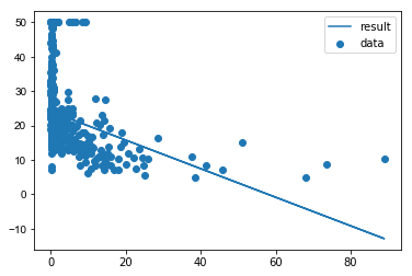
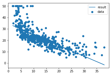
적합시킨 직선 시각화
import matplotlib.pyplot as plt
plt.yticks(fontname = "Arial") #
plt.scatter(crim,target,label="data")
plt.plot(crim,pred1,label="result")
plt.legend()
plt.show()
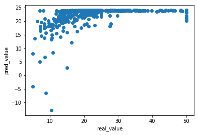
plt.scatter(target,pred1)
plt.xlabel("real_value")
plt.ylabel("pred_value")
plt.show()
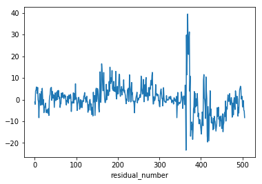
fitted_model1.resid.plot()
plt.xlabel("residual_number")
plt.show()
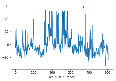
##잔차의 합계산해보기

sum(fitted_model1.resid)
-2.717825964282383e-13
위와 동일하게 rm변수와 lstat 변수로 각각 단순선형회귀분석 적합시켜보기
rm1 = sm.add_constant(rm, has_constant='add')
lstat1 = sm.add_constant(lstat, has_constant='add')
model2 = sm.OLS(target,rm1)
fitted_model2=model2.fit()
model3 = sm.OLS(target,lstat1)
fitted_model3=model3.fit()
fitted_model2.summary()
| Dep. Variable: | Target | R-squared: | 0.484 |
|---|---|---|---|
| Model: | OLS | Adj. R-squared: | 0.483 |
| Method: | Least Squares | F-statistic: | 471.8 |
| Date: | Mon, 12 Aug 2019 | Prob (F-statistic): | 2.49e-74 |
| Time: | 16:00:59 | Log-Likelihood: | -1673.1 |
| No. Observations: | 506 | AIC: | 3350. |
| Df Residuals: | 504 | BIC: | 3359. |
| Df Model: | 1 | ||
| Covariance Type: | nonrobust |
| coef | std err | t | P>|t| | [0.025 | 0.975] | |
|---|---|---|---|---|---|---|
| const | -34.6706 | 2.650 | -13.084 | 0.000 | -39.877 | -29.465 |
| RM | 9.1021 | 0.419 | 21.722 | 0.000 | 8.279 | 9.925 |
| Omnibus: | 102.585 | Durbin-Watson: | 0.684 |
|---|---|---|---|
| Prob(Omnibus): | 0.000 | Jarque-Bera (JB): | 612.449 |
| Skew: | 0.726 | Prob(JB): | 1.02e-133 |
| Kurtosis: | 8.190 | Cond. No. | 58.4 |
Warnings:
[1] Standard Errors assume that the covariance matrix of the errors is correctly specified.
fitted_model3.summary()
| Dep. Variable: | Target | R-squared: | 0.544 |
|---|---|---|---|
| Model: | OLS | Adj. R-squared: | 0.543 |
| Method: | Least Squares | F-statistic: | 601.6 |
| Date: | Mon, 12 Aug 2019 | Prob (F-statistic): | 5.08e-88 |
| Time: | 16:04:22 | Log-Likelihood: | -1641.5 |
| No. Observations: | 506 | AIC: | 3287. |
| Df Residuals: | 504 | BIC: | 3295. |
| Df Model: | 1 | ||
| Covariance Type: | nonrobust |
| coef | std err | t | P>|t| | [0.025 | 0.975] | |
|---|---|---|---|---|---|---|
| const | 34.5538 | 0.563 | 61.415 | 0.000 | 33.448 | 35.659 |
| LSTAT | -0.9500 | 0.039 | -24.528 | 0.000 | -1.026 | -0.874 |
| Omnibus: | 137.043 | Durbin-Watson: | 0.892 |
|---|---|---|---|
| Prob(Omnibus): | 0.000 | Jarque-Bera (JB): | 291.373 |
| Skew: | 1.453 | Prob(JB): | 5.36e-64 |
| Kurtosis: | 5.319 | Cond. No. | 29.7 |
Warnings:
[1] Standard Errors assume that the covariance matrix of the errors is correctly specified.
pred2=fitted_model2.predict(rm1)
pred3=fitted_model3.predict(lstat1)
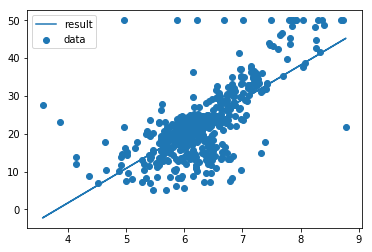
import matplotlib.pyplot as plt
plt.scatter(rm,target,label="data")
plt.plot(rm,pred2,label="result")
plt.legend()
plt.show()
import matplotlib.pyplot as plt
plt.scatter(lstat,target,label="data")
plt.plot(lstat,pred3,label="result")
plt.legend()
plt.show()
fitted_model2.resid.plot()
plt.xlabel("residual_number")
plt.show()
fitted_model3.resid.plot()
plt.xlabel("residual_number")
plt.show()
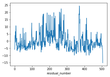
fitted_model1.resid.plot(label="crim")
fitted_model2.resid.plot(label="rm")
fitted_model3.resid.plot(label="lstat")
plt.legend()