NSMC 정제 - wordcloud 와 histogram으로 단어 분포 파악하기
NSMC 정제하기
-
Naver Sentiment Movie Corpus 영화 리뷰 학습을 통한 감정 예측 구현
-
감정분석을 위해, Naver Movie Corpus(https://github.com/e9t/nsmc/) 를 사용합니다.
def read_documents(filename):
    with open(filename, encoding='utf-8') as f:
        documents = [line.split('\t') for line in f.read().splitlines()]
        documents = documents[1:]

    return documents

train_docs = read_documents("ratings_train.txt")
test_docs = read_documents("ratings_test.txt")
print(len(train_docs))
print(len(test_docs))
150000
50000
함수 정의.
def text_cleaning(doc):
    # 한국어를 제외한 글자를 제거하는 함수.
    doc = re.sub("[^ㄱ-ㅎㅏ-ㅣ가-힣 ]", "", doc)
    return doc

def define_stopwords(path):

    SW = set()
    # 불용어를 추가하는 방법 1.
    # SW.add("있다")

    # 불용어를 추가하는 방법 2.
    # stopwords-ko.txt에 직접 추가

    with open(path) as f:
        for word in f:
            SW.add(word)

    return SW

def text_tokenizing(doc):
    return [word for word in mecab.morphs(doc) if word not in SW and len(word) > 1]

    # wordcloud를 위해 명사만 추출하는 경우.
    #return [word for word in mecab.nouns(doc) if word not in SW and len(word) > 1]
불러온 데이터를 품사 태그를 붙여서 토크나이징합니다.
from konlpy.tag import Mecab
from konlpy.tag import Okt
import json
import os
import re
from pprint import pprint

okt = Okt()
mecab = Mecab(dicpath='C:\mecab\mecab-ko-dic')

SW = define_stopwords("stopwords-ko.txt")

if os.path.exists('train_docs.json'):
    with open("train_docs.json", encoding='utf-8') as f:
        train_data = json.load(f)
else:
    train_data = [(text_tokenizing(line[1]), line[2]) for line in train_docs if text_tokenizing(line[1])]
#     train_data = []
#     for line in train_docs:
#         if text_tokenizing(line[1]):
#             train_data.append((text_tokenzing(line[1]), line[2]))


    with open("train_docs.json", 'w', encoding='utf-8') as f:
        json.dump(train_data, f, ensure_ascii=False, indent='\t')

if os.path.exists('test_docs.json'):
    with open("test_docs.json", encoding='utf-8') as f:
        test_data = json.load(f)
else:
    test_data = [(text_tokenizing(line[1]), line[2]) for line in test_docs if text_tokenizing(line[1])]

    with open("test_docs.json", 'w', encoding='utf-8') as f:
        json.dump(test_data, f, ensure_ascii=False, indent='\t')

pprint(train_data[0])
pprint(test_data[0])
(['진짜', '짜증', '네요', '목소리'], '0')
(['GDNTOPCLASSINTHECLUB'], '0')
NLTK를 이용한 histogram 분석.
-
데이터 분석을 하기 위해 기본적인 정보들을 확인합니다.
-
nltk 라이브러리를 이용하여 전처리를 합니다.
import nltk

total_tokens = [token for doc in train_data for token in doc[0]]
print(len(total_tokens))
1206841
- example
v = [list(range(10)),[10,11,12]]
print(v)
[[0,1,2,3,4,5,6,7,8,9],[10,11,12]]
for i in v:
  for j in i:

      print(j)
[j for i in v for j in i]
[0,1,2,3,4,5,6,7,8,9,10,11,12]
-
example 2
for doc in train_data
 for token in doc[0]

     print(token)
[token for doc in train_data for token in doc[0]]
*모든 데이터가 모두 출력된다
text = nltk.Text(total_tokens, name='NMSC')
print(len(set(text.tokens)))
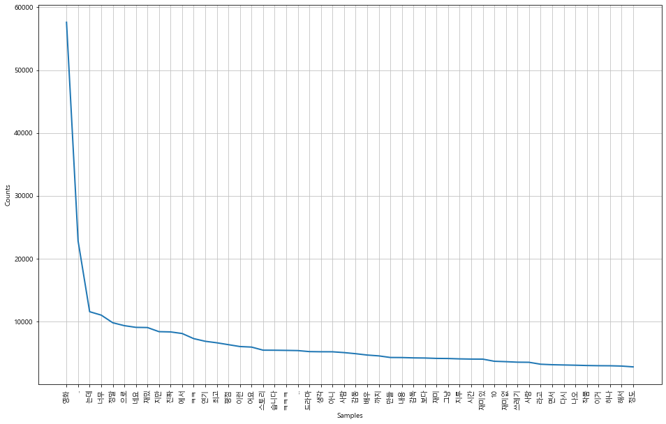
pprint(text.vocab().most_common(10))
51722
[('영화', 57614),
 ('..', 22813),
 ('는데', 11543),
 ('너무', 11002),
 ('정말', 9783),
 ('으로', 9322),
 ('네요', 9053),
 ('재밌', 9022),
 ('지만', 8366),
 ('진짜', 8326)]
Histogram 그리기.
import matplotlib.pyplot as plt
import platform
from matplotlib import font_manager, rc
%matplotlib inline

path = "c:/Windows/Fonts/malgun.ttf"
if platform.system() == 'Darwin':
    rc('font', family='AppleGothic')
elif platform.system() == 'Windows':
    font_name = font_manager.FontProperties(fname=path).get_name()
    rc('font', family=font_name)
else:
    print('Unknown system... sorry~~~~')

plt.figure(figsize=(16, 10))
text.plot(50)
WordCloud 그리기.
from wordcloud import WordCloud

data = text.vocab().most_common(100)

# for win : font_path='c:/Windows/Fonts/malgun.ttf'
wordcloud = WordCloud(font_path='c:/Windows/Fonts/malgun.ttf',
                      relative_scaling = 0.2,
                      #stopwords=STOPWORDS,
                      background_color='white',
                      ).generate_from_frequencies(dict(data))
plt.figure(figsize=(16,8))
plt.imshow(wordcloud)
plt.axis("off")
plt.show()